When you are working with a spreadsheet that has subtotals you created by selecting Data » Subtotals (see, Insert Subtotals For a Range of Data), the subtotals can be very hard to identify, making the spreadsheet hard to read. This is true especially if you applied subtotals to a table of data with many columns.
Typically, the resulting subtotals appear on the right, while their associated headings are often in the first column. As the subtotal values are not in boldface, it can be hard to visually align them with their row headings. You can make these subtotals much easier to read by applying bold formatting to the subtotal values and by highlighting the data row.
To test the problem, set up some data similar to that shown in the figure.
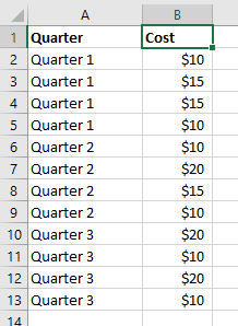
Now add the subtotals by selecting Data » Subtotals, accepting the defaults in the Subtotals dialog, and clicking OK.
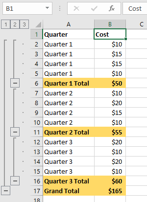
In the figure, the subtotal headings have been boldfaced but their associated results have not. As this table has only two columns, it is not that hard to read and pick out the subtotal amounts.
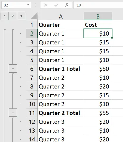
The more columns a table has, however, the harder it is to visually pick out the subtotals. You can solve this problem by using Excel’s conditional formatting. Using the table in from figure as an example, try this before adding your Subtotals:
- Select cell
A1:B13, ensuring thatA1is the active cell. - Go to the
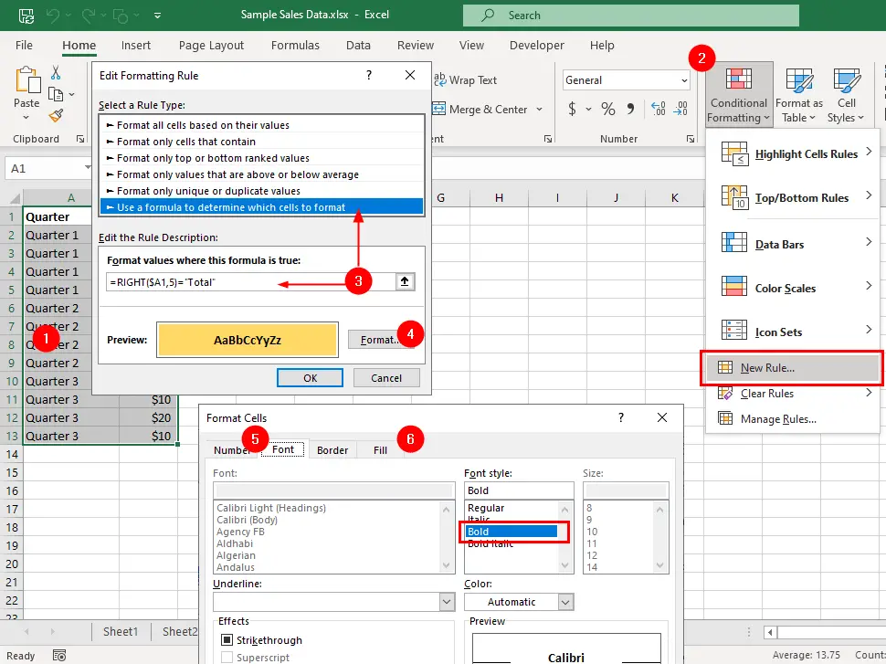
Hometab, clickConditional Formattingdrop-down, and chooseNew Rule..., it will opens theNew Formatting Ruledialog box. - Select
Use a formula to determine which cells to formatfrom the Select a rule type box, and then add the following formula:
=RIGHT($A1,5)="Total"
- Now click the
Formatbutton. - And then the
Fonttab, and selectBoldas theFont Style. - Next, click the
Filltab and select a color from theBackground Colorsection. - Click
OK, thenOKagain.
The important part of the formula is the use of an absolute reference of the column $A and a relative reference of the row 1. As you start the selection from cell A1, Excel will automatically change the formula for each cell.
For example, cells A2 and B2 will have the conditional format formula =RIGHT($A2,5)="Total“, and cells A3 and B3 will have the conditional format formula =RIGHT($A3,5)="Total“.
Add the subtotals, and they will look like those in the figure.
One last thing to remember is that if you remove the subtotals, the formatting will no longer apply.
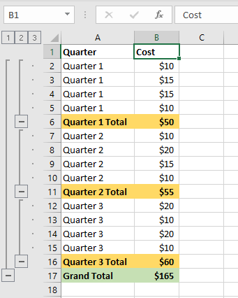
The only possible pitfall with this method is that the Grand Total appears in the same style as the Subtotals. It would be nice to see the Grand Total formatted in another way so that it stands out from the Subtotals and is identified more easily. You can do this using the same example.
Starting with your raw data, select cell A1:B13, ensuring that A1 is the active cell. Create a second conditional formatting and in step 3, add the following formula:
=$A1="Grand Total"
Click the Format button and then the Font tab, and select Bold as the Font Style. Click the Fill tab and select a different background color. Click OK, and then click OK again.
Next, select Data » Subtotals, accept the defaults, and click OK. Your worksheet data should now look like the figure.
You can use any format you want to make your subtotals easier to read.