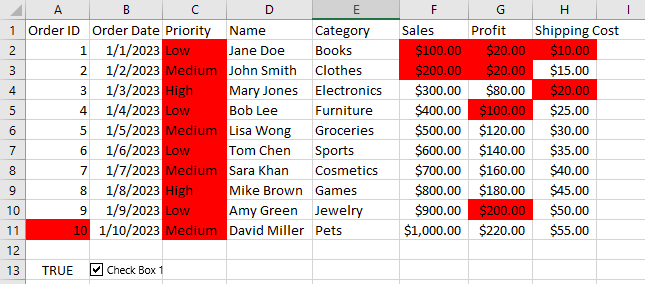
For this example, you’ll apply conditional formatting to a range of cells so that any data appearing more than once is highlighted for easy identification. We’ll assume your table of data extends from cell $A$1:$H$11. To conditionally format this range of data so that you can identify duplicates requires a few steps.
1. Enable Developer Tab
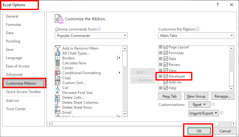
If the Developer tab is not already showing, right-click any tab and select Customize the Ribbon, then check the Developer from the Main Tabs box and click OK.
2. Insert a Checkbox to Turn Conditional Formatting On and Off
- Go to the
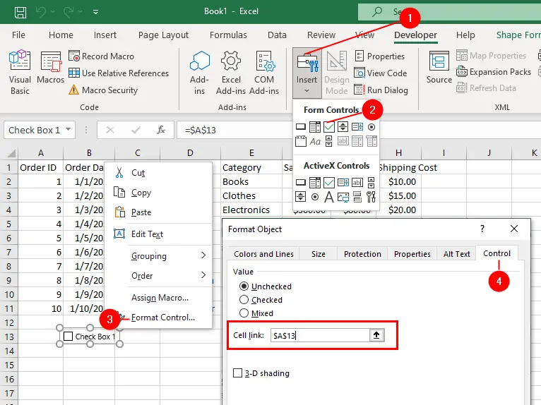
Developertab and click onInsertin the Controls group. - Select the
Checkboxoption from the Form Controls section. - Right-click the checkbox and select
Format Control. - Select the
Controltab and in the Cell Link box, type$A$13and click OK.
For more information, visit Setting Up Checkboxes for Conditional Formatting.
3. Apply Conditional Formatting
- Select cell
A2, then drag and select a range down to cellH11. It is important that cellA2is the active cell in your selection. - Select
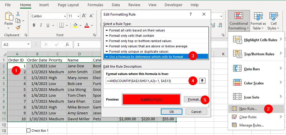
Home » Conditional Formatting » New Rule. - Select Use a formula to determine which cells to format.
- Type
=AND(COUNTIF($A$2:$H$11,A2)>1,$A$13)in the “Format values where this formula is true” box. - Click on
Formatand select a color you want to be applied to duplicated data. Click OK, then OK again.
Although the checkbox you added to the worksheet is checked, the cell link in $A$13 will read TRUE and all duplicates within the range $A$2:$A$11 will be highlighted. As soon as you deselect the checkbox, its cell link ($A$13) will return FALSE, and duplicates will not be highlighted.
The checkbox gives you a switch so that you can turn conditional formatting on and off from the spreadsheet, with no need to return to the Conditional Formatting dialog box. You can apply the same principle to data validation when using the formula option.
This works because you used the AND function. AND means two things must occur: COUNTIF($A$2:$H$11,A2)>1 must return TRUE, and the cell link for the checkbox ($A$13) also must be TRUE. In other words, both conditions must be TRUE for the AND function to return TRUE.
Conditional Formatting
- Setting Up Checkboxes for Conditional Formatting
- Highlighting Formula Cells with Conditional Formatting
- Sum Cells That Meet Conditional Formatting Criteria
- Highlight Every Other Row or Column with MOD Function and Conditional Formatting
- Enable and Disable Conditional Formatting with a Checkbox
- Sort Data By Conditional Formatting Criteria