Raised Effect
To start off with a simple example, we’ll give a cell a 3D effect so that it appears raised, like a button. On a clean worksheet follow these steps to create the effect:
- Select cell
D5(because it’s not on an edge). - Select
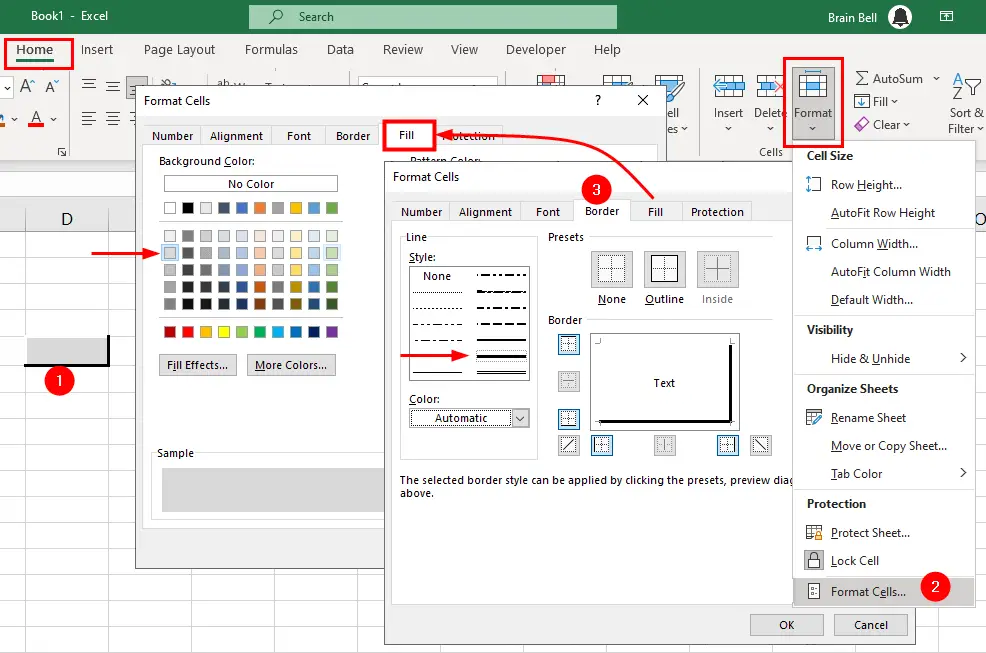
Home » Format » Format Cells. - Go to the
Bordertab and from the Line box, choose the second thickest line style. - Ensure that the color selected is Black (or Automatic, if you haven’t changed the default for this option).
- Now click the righthand border and then click the bottom border.
- Select white from the color drop-down.
- The second thickest border still should be selected, so this time click the two remaining borders of the cell, the top border and the left border.
- Click the
Filltab on the Format Cells dialog and make the cell shading Gray. - Click OK and deselect cell
D5.
Cell D5 will have a raised effect that gives the appearance of a button. You did it all with borders and shading.
Pushed or indented Effect
If, for fun or diversity, you want to make a cell look indented or pushed in, follow these steps:
- Select cell
E5(because it’s next toD5and it makes the next exercise work). - Select
Home » Format » Format Cells. - Go to the
Bordertab and from the Line box, choose the second thickest line style. Ensure that the color selected is Black (or Automatic, if you haven’t changed the default for this option). - Apply the formatting to the top and left border of the cell.
- Select white from the color drop-down.
- The second thickest border still should be selected, so this time click the two remaining borders of the cell, the bottom border and the right border.
- Click the
Filltab on the Format Cells dialog and make the cell shading Gray. - Click OK and deselect cell
E5.
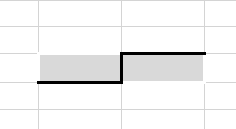
Cell E5 should appear indented. This works even better in contrast with cell D5, which has the raised effect.
Using a 3D Effect on a Table of Data
Next, we’ll experiment with this tool to see the sorts of effects you can apply to your tables or spreadsheets to give them some 3D excitement.
- Select cells
D5andE5 - click the
Format Paintertool (the paintbrush icon) on the Home tab. - While holding down the left mouse button, click on cell
F5, drag across to cellJ5and release. - Now select cells
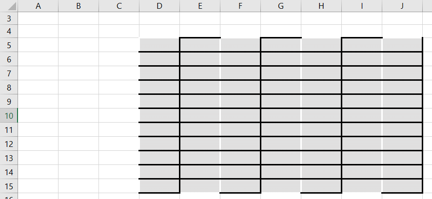
D5:J5and again click theFormat Paintertool on the Home tab. - While holding down the left mouse button, select cell
D6and drag it across and down to cellJ15, then release. - This should produce the effect shown in the figure.
We have used a fairly thick border to ensure that the effect is seen clearly; however, you might want to make this a little subtler by using a thinner line style. You also could use one of the other line styles to produce an even greater effect. The easiest way to find good combinations is to use trial and error on a blank worksheet to create the effect you want. You are limited only by your imagination and, perhaps, your taste.