- Create Custom Number Format
- Understanding Format Code Sections
- List of Formatting Codes
- Apply Conditions and Color in Custom Number Format
The default format for any cell is General. If you enter a number into a cell, Excel often will guess the number format that is most appropriate. For example, if you enter 10% into a cell, Excel will format the cell as a percentage. Most of the time, Excel guesses correctly, but sometimes you need to change it. By default, numbers are right-aligned and text is left-aligned. If you leave this alone, you can tell at a glance whether a cell is text or numeric.
Create Custom Number Format
To create a custom number format, follow these steps:
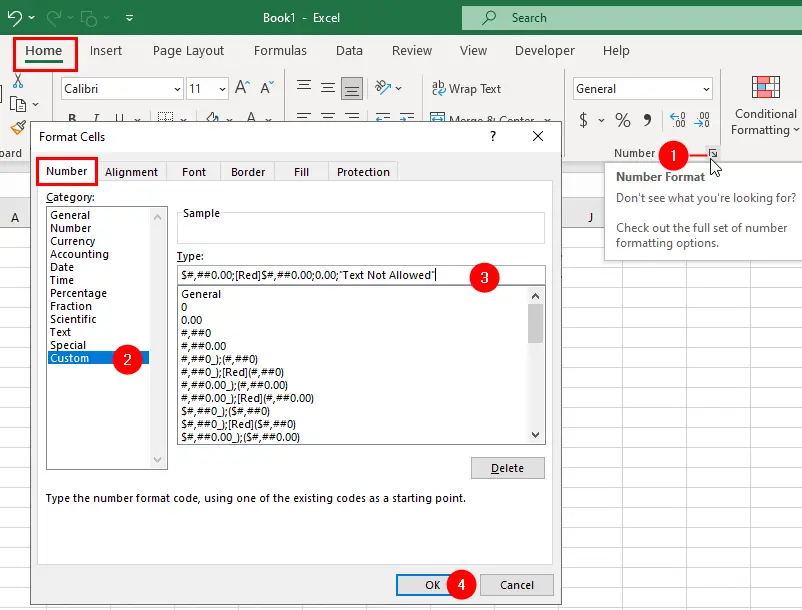
- On the
Hometab, click theNumberdialog box launcher in theNumbergroup.
Or, right-click the cell/range that you want to format and clickFormat Cellsfrom the context menu. - The
Format Cellsdialog box will appear. Click theNumbertab and chooseCustomfrom the Category list. - In the
Typebox, write the format code that you want to use. You can also use one of the predefined codes. For example:0.00: Display a number with two decimal places:#,##0.00: Display a number with the thousand separators and two decimal places.[Green]0.00;[Red]-0.00: Display positive numbers in green and negative numbers in red.0.0,"K": Display large numbers in thousands with aKsuffix.0.00%: Display a percentage with two decimal places.
- Click
OKto apply the format to selected cells.
The format codes consist of sections separated by a semicolon ;, where each section represents how positive numbers, negative numbers, zeros, and text values should be formatted.
Understanding Format Code Sections
Excel format codes are a way of customizing how numbers, dates, times, fractions, percentages, and other values are displayed in a cell. They consist of a combination of symbols and placeholders that define the appearance of the value.
For example, the format code #,##0.00 displays a number with a thousand separator and two decimal places. The format code m/d/yyyy displays a date with slashes as separators and four digits for the year.
Excel sees a cell’s format as having four sections (from left to right). Each section is separated by a semicolon ;:
- Positive Numbers,
- Negative Numbers,
- Zero Values, and
- Text Values.
When you create a custom number format, you do not have to specify all four sections. If you include only two sections, the first section will be used for both positive numbers and zero values, while the second section will be used for negative numbers. If you include only one section, all number types will use that one format. Text is affected by custom formats only when you use all four sections; the text will use the last section.
Each section of a given format uses its own set of formatting codes. These codes force Excel to make data appear how you want it to appear. So, for instance, suppose you want negative numbers to appear inside parentheses, and all numbers, positive, negative, and zero, to show two decimal places. To do this, use this custom format:
0.00;(-0.00)If you also want negatives to show up in red, use this custom format:
0.00;[Red](-0.00)Note the use of the square brackets in the preceding code. The formatting code tells Excel to make the number red.
Let’s create a number format that you can customize to meet your needs:
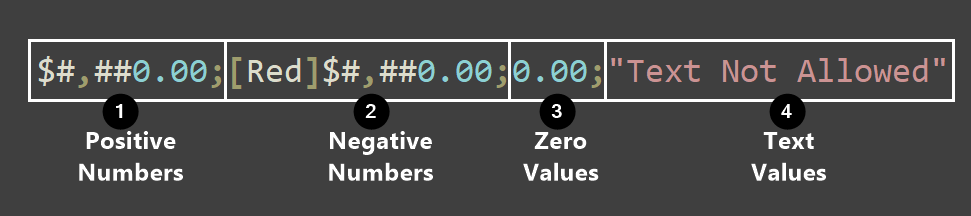
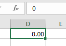
$#,##0.00;[Red]$#,##0.00;0.00;"Text Not Allowed"The custom number format shown above is Excel’s standard currency format, which shows negative currencies in red. We modified it by adding a separate format for zero values and another one for text.
If you enter a positive number as a currency value, Excel will format it automatically so that it includes a comma for the thousands separator, followed by two decimal places. See figure:
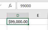
99000 shows up with the leading dollar sign, comma for the thousands separator, and followed by two decimal placesIt will do the same for negative values, except they will show up in red. See figure:

-99000 shows up in redAny zero value will have no currency symbol and will show two decimal places. See figure:
If you enter text into a cell, Excel will display the words “Text Not Allowed” regardless of the true underlying text. See figure:
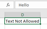
Hello) will show up “Text Not Allowed”List of Formatting Codes
Now, you can create your custom number format using a combination of formatting codes. Here are some common formatting codes:
- Number Codes:
General: General number format.0: A placeholder for a digit (leading zeros will be displayed).#: A placeholder for a digit (leading zeros will be suppressed).?: A placeholder for a single digit (extra spaces will be used for shorter numbers).%: A percentage. Excel multiplies by 100 and displays the % character after the number.,: (Comma) A thousands separator. A comma followed by a placeholder scales the number by1,000.E+ E- e+ e-: Scientific notation.
- Decimal Places Codes:
.0: Display one decimal place..00: Display two decimal places..000: Display three decimal places.
- Text and Symbols Codes:
"text": Display text within double quotes.$ - + / ( )and blank space: These characters are displayed in the number, no need to enclose them in quotation marks or precede them with a backslash.\: Escape character, used to display characters like,,",*,!,^,&,',~,{,},=,<, or>.*: This code repeats the next character in the format to fill the column width. Only one asterisk per section of a format is allowed._; This code skips the width of the next character. This code is commonly used as_)to leave space for a closing parenthesis in a positive number format when the negative number format includes parentheses. This allows both positive and negative values to line up at the decimal point.@: A placeholder for text.
- Dates Codes:
d: A day represented without leading zeros (1-31)
dd: A day represented with leading zeros (01-31)ddd: A weekday represented as an abbreviation (Sun-Sat)dddd: An unabbreviated weekday name (Sunday-Saturday)m: Month as one or two digits.mm: Month as two digits.mmm: Abbreviated month name (e.g., Jan, Feb, Mar).mmmm: Full month name (e.g., January, February, March).yy: Two-digit year (for example, 23).yyyy: Four-digit year (for example, 2023).
- Time Codes:
h: Hour without leading zeros (24-hour clock).
hh: Hour with leading zeros (24-hour clock).m: Minute without leading zeros (0-59).mm: Minute with leading zeros (00-59).s: Second without leading zeros (0-59).ss: Second with leading zeros (00-59).AM/PM am/pm: Time of day based on a 12-hour clock
- Color and Conditions
[BLACK],[BLUE],[CYAN],[GREEN],[MAGENTA],[RED],[WHITE],[YELLOW],[COLOR n]:
These codes display characters in the specified colors. Note thatnis a value from1to56and refers to the nth color in the color palette.[Condition value]:
Condition can be<,>,=,>=,<=, or<>, while value can be any number. A number format can contain up to two conditions.
Apply Conditions and Color in Custom Number Format
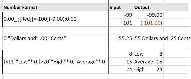
Note in particular the last kind of formatting codes in the above table: colors and comparison operators. Assume you want the custom number format 0.00_ ;[Red](-0.00) to display negative numbers in a red font and in brackets only if the number is less than -100. To do this, use the following:
0.00_ ;[Red][<-100](-0.00);0.00
The formatting codes [Red][<-100](-0.00) placed in the section for negative numbers make this possible. Using this method in addition to conditional formatting you can double the number of conditional format conditions available from three to six.
Often, users want to display dollar values as words. To do this, use the following custom format:
0 "Dollars and" .00 "Cents"
This format will force a number entered as 55.25 to be displayed as 55 Dollars and .25 Cents.
You can also use a custom format to display the words Low, Average, or High, along with the number entered. Simply use this formatting code:
[<11]"Low"* 0;[>20]"High"* 0;"Average"* 0
Note the use of the *. This repeats the next character in the format to fill the column width, meaning that all the Low, Average, or High text will be forced to the right, while the number will be forced to the left.