Here is an example of how to do it.
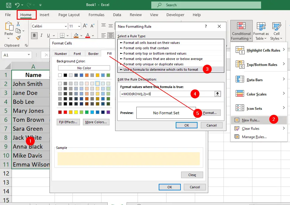
- Select the range of cells that you want to format.
- Click
Home > Conditional Formatting > New Rule. - Select
Use a formula to determine which cells to formatfrom the New Formatting Rule dialog box - In the
Format values where this formula is truebox, enter one of these formulas:- To highlight every other row, use
=MOD(ROW(),2)=0 - To highlight every other column, use
=MOD(COLUMN(),2)=0
- To highlight every other row, use
- Click
Formatbutton and choose the fill color that you want from theFilltab. - Click OK to close the Format Cells dialog box and then click OK again to apply the rule.
Apply color to alternate rows or columns dynamically
Although the above method applies the formatting specified to every second row or column quickly and easily, it is not dynamic. Rows containing no data will still have the formatting applied. This looks slightly untidy and makes reading the spreadsheet a bit more difficult. Making the highlighting of every second row or column dynamic takes a little more formula tweaking:
- Again, select the range, for example,
A1:E15. - Click
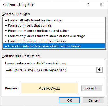
Home > Conditional Formatting > New Rule. - Select
Use a formula to determine which cells to formatfrom the New Formatting Rule dialog box - In the
Format values where this formula is truebox, enter this formula:=AND(MOD(ROW( ),2),COUNTA($A1:$E1)) - Click
Formatbutton and choose the fill color that you want from theFilltab. - Click OK to close the Format Cells dialog box and then click OK again to apply the rule.
Note that you do not reference rows absolutely (with dollar signs), but you do reference columns this way.
Any row within the range A1:E15 that does not contain data will not have conditional formatting applied. If you remove data from a specific row in your table, it too will no longer have conditional formatting applied. If you add new data anywhere within the range A1:E15, the conditional formatting will kick in.

This works because when you supply a formula for conditional formatting, the formula itself must return an answer of either TRUE or FALSE. In the language of Excel formulas, 0 has a Boolean value of FALSE, while any number greater than zero has a boolean value of TRUE. When you use the formula =MOD(ROW( ),2), it will return either a value of 0 (FALSE) or a number greater than 0.
The ROW( ) function is a volatile function that always returns the row number of the cell it resides in. You use the MOD function to return the remainder after dividing one number by another. In the case of the formula you used, you are dividing the row number by the number 2, so all even row numbers will return 0, while all odd row numbers will always return a number greater than 0.
When you nest the ROW( ) function and the COUNTA function in the AND function, it means you must return TRUE (or any number greater than 0) to both the MOD function and the COUNTA function for the AND function to return TRUE. COUNTA counts all nonblank cells.
Conditional Formatting
- Setting Up Checkboxes for Conditional Formatting
- Highlighting Formula Cells with Conditional Formatting
- Sum Cells That Meet Conditional Formatting Criteria
- Highlight Every Other Row or Column with MOD Function and Conditional Formatting
- Enable and Disable Conditional Formatting with a Checkbox
- Sort Data By Conditional Formatting Criteria