The GETPIVOTDATA function is used to extract data from a pivot table based on specified criteria. The syntax of the function is:
GETPIVOTDATA(data_field, pivot_table, [field1, item1, field2, item2], …)data_fieldname of the value field to query.pivot_tablea reference to any cell in the pivot table.[field1, item1...]optional field and item arguments. These are the pairs of criteria that specify which subset of data to retrieve. For example:field1could beCategoryanditem1could beCategory Name.field2could be Country anditem2could beUnited States.
To use this function, type = (an equals sign) in any cell, and then use your mouse pointer to click on the cell in the pivot table currently housing your desired value, e.g. Total Profit. Excel will automatically fill in the arguments for you.
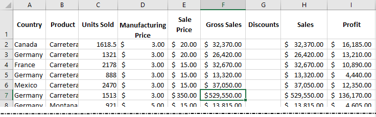
Here are some examples of how to use this function. We used the following data table to create the pivot table for our examples:
And we created the following pivot table from the data:
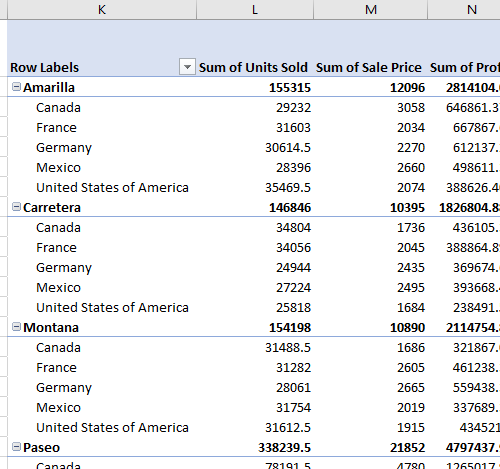
To get the total profit amount for a specific product (e.g. Paseo), you can use the following formula:
=GETPIVOTDATA("Profit",K1,"Product","Paseo")This formula returns the value of the Profit field for the item Paseo in the PivotTable located at the cell K1.
To get the sum of profit for all products, you can use one of the following formulas:
- Use the field name Profit from the data table
=GETPIVOTDATA("Profit",K1)- OR use the field name Sum of Profit from Pivot Table
=GETPIVOTDATA("Sum of Profit",K1)Move PivotTable Grand Totals
One of the most annoying things about PivotTables is that the Grand Total that summarizes your data always ends up at the bottom of the table, meaning you have to scroll down just to see the figures. Move your Grand Total up to the top where it’s easier to find.
Although PivotTables are a great way to summarize data and extract meaningful information, there is no built-in option to have the Grand Total float to the top for a quick bird’s-eye view.
Before we describe a very generic method to move the Grand Total to the top, we’ll explain how you can accomplish this with the GETPIVOTDATA function, which is designed specifically to extract data from a PivotTable.
You can use the function like this:
=GETPIVOTDATA("Sum of Sale Price",$K$1)or like this:
=GETPIVOTDATA("Sale Price",$k$1)Either function will extract the data and will track the Grand Total as it moves up, down, left, or right. We used the cell address $K$1, but as long as you use any cell within the PivotTable, you always will pick up the total.
Note: The first function uses the Sum of Sale Price field, while the second one uses the Sale Price field:
- If your PivotTable has the
Sale Pricefield in the Data table, you need to name the fieldSale Price. - If, however, the
Sale Pricefield is being used two or more times in the pivot table, you must specify the name you gave it in the pivot table.