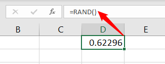
RAND() Function
Excel RAND() function generates a random decimal number between 0 and 1. Type RAND() in the cell where you want the random number to appear, Excel will generate a random decimal number between 0 and 1 in the selected cell.
The RAND function is a volatile function that will recalculate automatically whenever an action takes place in Excel e.g., entering data somewhere else, or forcing a recalculation of the worksheet by pressing F9.
You can copy and paste the formula to other cells to generate additional random numbers.
If you want to generate a new random number, you can press F9 or recalculate the worksheet. It’s important to note that each time the worksheet is calculated, all instances of the RAND function will be recalculated, resulting in different random numbers. If you want to keep the generated random numbers static, you can use the Paste Special feature to convert the formulas to values.
Generate Random Number Between 1 and 100
If you want to generate random numbers within a specific range, you can use formulas to manipulate the random numbers generated by the RAND() function. Assume you want to generate random whole numbers between 1 and 100. Here’s the formula:
=INT( RAND() * 100 ) + 1
Here’s how it works:
- The
RAND()function generates a random decimal number between 0 and 1. RAND()*100:
We multiply the random decimal number generated byRAND()by100. This step scales the random number to a range between0and100.- The
INT()function rounds down a number to the nearest integer. In this case, it ensures that the decimal portion of the multiplied random number is discarded, giving us a whole number between0and99. - We add
1to the result of theINT()function. This shifts the range of the generated random number from0-99to1-100. So, the final result will be a random whole number between1and100.
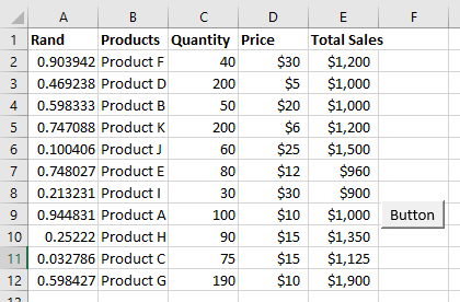
Random Sort
Assume you have a three-column table in your spreadsheet, starting from column B. You can place the RAND() function in cell A2 and copy this down as many rows as needed, all the way to the end of your table. As soon as you do this, each cell in column A containing the RAND function will automatically return a random number by which you can sort the table. In other words, you can sort columns A, B, C, and D by column A in either ascending or descending order.
The RAND function is a volatile function, you can use this volatility to your benefit and record a macro that sorts data immediately after you recalculate and force the RAND function to return another set of random numbers. You then can attach this macro to a button so that each time you want to shuffle (random sort) data, all you need to do is click the button.
For example, assume you have your data in columns B, C, and D and that row 1 is used for headings:
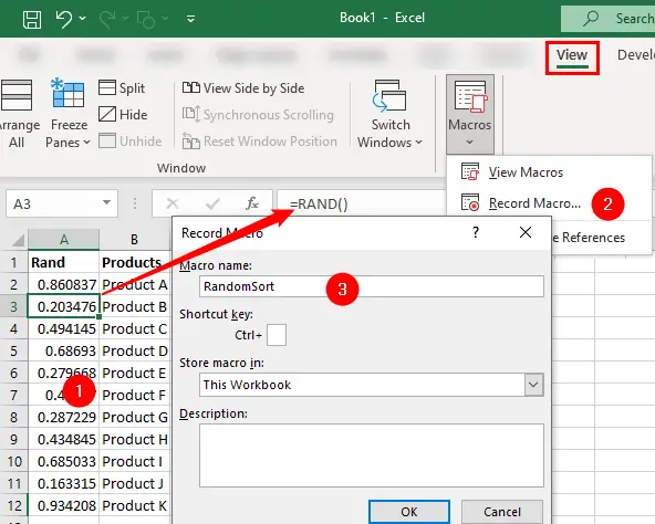
- First, place the heading
RANDin cellA1. Enter=RAND( )in cellA2and copy down as far as needed. - Then select any single cell and select
View » Macro » Record Macro. It will open theRecord Macrodialog box. - Assign the macro a name i.e.
RandomSortand click OK button, see the following figure:
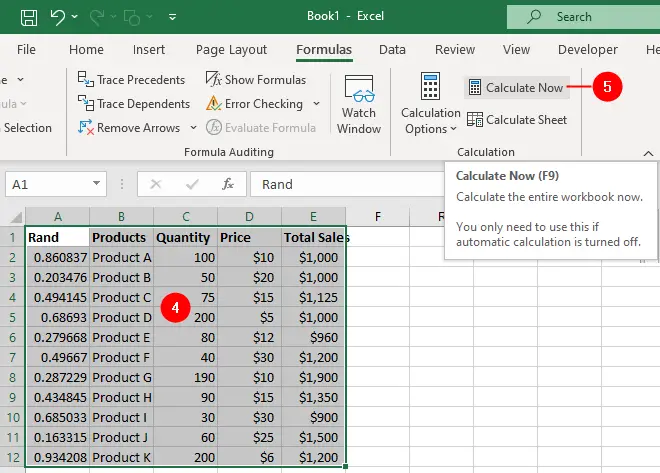
- Select columns
A,B,C, andD - Click
Formula » Calculate Nowbutton (or pressF9) to force a recalculation.
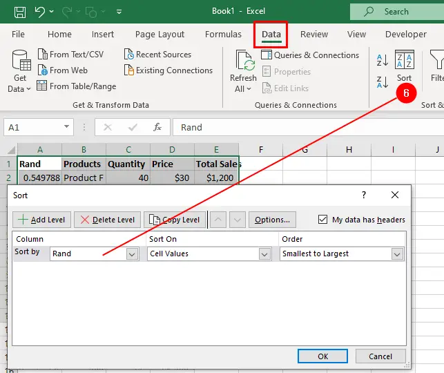
- Select
Data » Sortand sort the data by columnA.
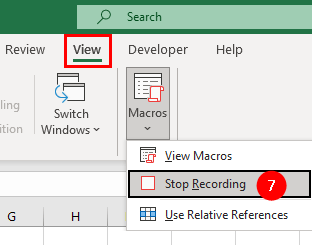
- Stop recording the macro by clicking the
View » Macrosdrop-down.
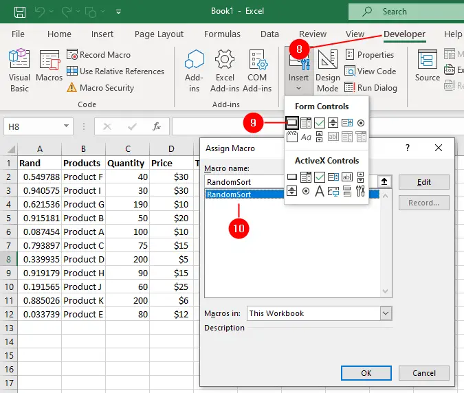
- Next, click
Developer » Insertin theControlsgroup. - Click the
Buttonicon from theForms Controls. - The Assign Macro dialog box will appear, assign the macro you just recorded to this button and click OK.
- Place the button anywhere on the worksheet.
Each time you click the button, your data will be sorted randomly. You can select column A and hide it completely, as there is no need for a user to see the random numbers generated.