Creating a PivotTable in Excel is a relatively straightforward process. First, prepare the data to use in the PivotTable. Ensure that your data is well-structured with column headers. Each column should have a header that describes the data in that column. In this section, you’ll also create a pivot table from another workbook.
Here are the steps to create a pivot table:
- Click anywhere within your dataset.
- Go to the
Inserttab in the ribbon. - Click on the
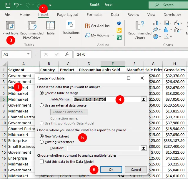
PivotTablebutton. This opens the “Create PivotTable” dialog box. - In the “Create PivotTable” dialog box, Excel will automatically detect the data range you selected.
- Choose one of the following options to place the PivotTable:
New Worksheet: This option creates a new worksheet for the PivotTable.Existing Worksheet: This option allows you to specify an existing worksheet location for the PivotTable. Simply click the location in your worksheet where you want the PivotTable to begin.
- Click OK.
Excel inserts the new pivot table as an empty placeholder. You need to tell Excel what data to put into this table. You do this by choosing which columns from your original data should be used for the rows, columns, and values in the PivotTable. These columns will determine how your data is summarized and organized. You can choose these columns from the PivotTable Field List on the right side of the window.
In the PivotTable Field List, you’ll see a list of fields from your dataset. Drag and drop fields into the following areas:
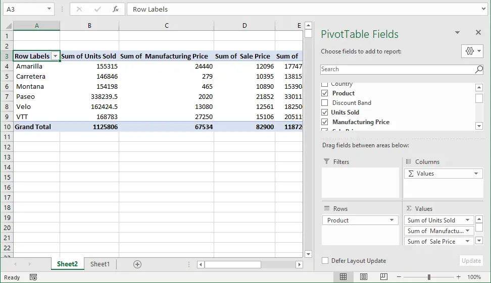
- Rows: This is where you define the criteria or categories you want to use for row labels.
- Columns: This is where you define the criteria or categories you want to use for column labels.
- Values: This is where you specify what data you want to summarize (e.g., sum, count, average).
- Filters: This is where you can apply filters to limit the data displayed in your PivotTable.
If your source data changes, you can refresh the PivotTable to update it. Right-click inside the PivotTable and select Refresh.
External Data Sources: Pull Data From Another Workbook
Follow these steps to create a pivot table using data from an external source or from another workbook:
- Go to the
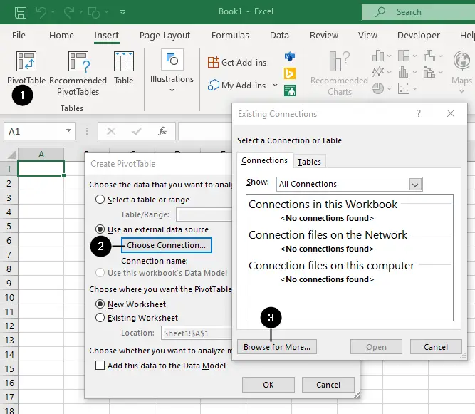
Inserttab and click on thePivotTablebutton. - Choose
Use an external data sourceand click onChoose Connectionin the “Create PivotTable” dialog box. - Click
Browse for Morebutton and browse for the workbook you want to use as the data source and click Open as shown in the figure:
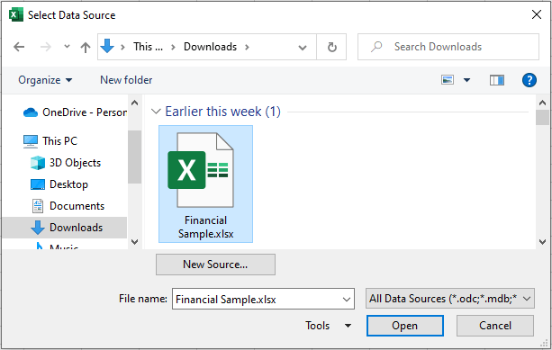
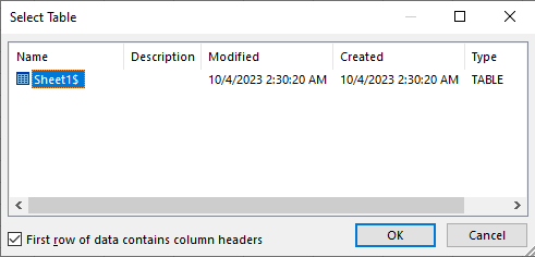
Excel will display the “Select Table” dialog box that lists all tables in the selected workbook. Choose the table that you want to use for the pivot table and click OK.
Click OK again to close the Create PivotTable dialog box.
Excel inserts the new pivot table as an empty placeholder. You need to tell Excel what data to put into this table, or you can use Recommended PivotTables features to automatically create pivot tables from the source data.
Recommended PivotTables
The Recommended PivotTables feature is a useful way to quickly create PivotTables without having to manually set up the fields. Excel analyzes your data and suggests PivotTable layouts that it believes will help you gain insights from your data efficiently. You can always make adjustments and add or remove fields as needed to refine your analysis.
Here’s how to use it:
- If you’ve not yet run the PivotTable wizard:
Click anywhere on the data, go to theInserttab and click theRecommended PivotTablesbutton. - If you’ve already inserted the PivotTable:
Go toPivotTable Analyzetab and click theRecommended PivotTablebutton, as shown in the following figure:
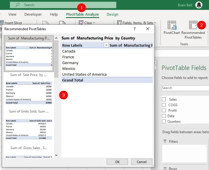
Review the list of recommended PivotTables provided by Excel. Each recommendation will have a brief description, and you can see a preview of how your data will look in the PivotTable. Select the one that best suits your analysis needs and click OK.