Make Animated Chart using Named Ranges and VBA

To begin, insert a bar or line chart using some data similar to that shown in the figure:

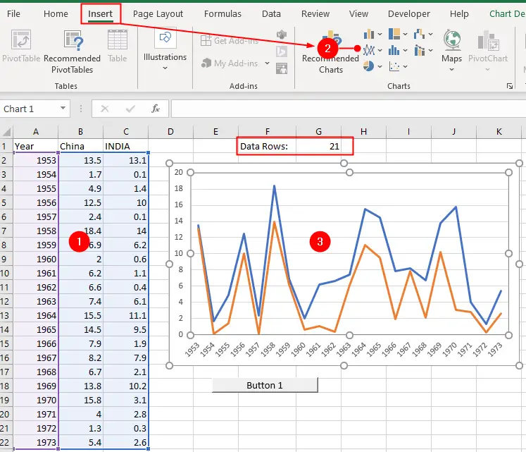
The value entered in cell G1, labeled “Data Rows”, dictates the number of records displayed on the chart. The value in cell G1 will be used by named ranges that we create in the next step.

2. Create Dynamic Named Ranges

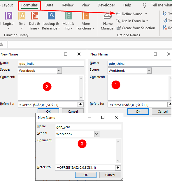
Next, create a three dynamic named ranges by selecting Formulas » Define Name and repeating the following steps:

1. In the Name: box type gdp_china and
   in the Refers to: box, type =OFFSET($B$2,0,0,$G$1,1)
2. In the Name: box type gdp_india and
   in the Refers to: box, type =OFFSET($C$2,0,0,$G$1,1)
3. In the Name: box type gdp_year and
   in the Refers to: box, type =OFFSET($A$2,0,0,$G$1,1)

Read Create Scrollable Charts tutorial to learn more about the dynamic ranges.

3. Use Named Ranges in Data Series

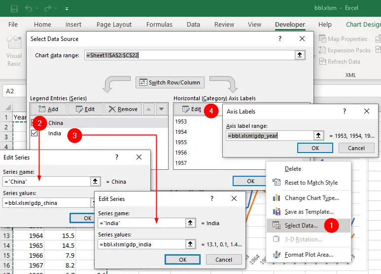
1. Right click on the chart and click Select Data option from the context menu.
   Remove all existing entries from the Legend Entries (Series) tab except China and India.
2. Select China and click Edit button, the Edit Series dialog appears:
   type China in the Series name box
   type =workbookName.xlsm!gdp_china in the Series values box
   click OK.
3. Select India and click Edit button, the Edit Series dialog appears:
   type India in the Series name box
   type =workbookName.xlsm!gdp_india in the Series values box
   click OK.
4. Click Edit button in Horizontal (Category) Axis Labels tab. The Axis Labels dialog box appears.
   type =workbookName.xlsm!gdp_year in the Axis label range box and
   click OK.
5. Again click OK button to close the Select Data Source dialog box.

4. Create Macros to Animate Chart Progress

Next we create a macro that will change the value of cell G1 dynamically. Press Alt + F11 to open the Visual Basic for Applications (VBA) editor and go to Insert > Module to insert a new module.

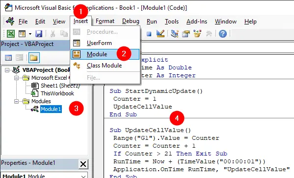
Copy and paste the following code into the module window:

Option Explicit
Dim RunTime As Double
Dim Counter As Integer

Sub StartDynamicUpdate()
 Counter = 1
 UpdateCellValue
End Sub

Sub UpdateCellValue()
 Range("G1").Value = Counter
 Counter = Counter + 1
 If Counter > 21 Then Exit Sub
 RunTime = Now + (TimeValue("00:00:01"))
 Application.OnTime RunTime, "UpdateCellValue"
End Sub

This code will update the value of cell G1 once in a second, starting from 1 and stopping when the value reaches 21. Adjust the interval (TimeValue("00:00:01")) if you want to change the update frequency.

Close the VBA editor.

5. Run Your VBA Code To Update Chart Data Dynamically

Once your macro is saved, you can run it by going back to the Developer tab, clicking on Macros, selecting the macro you want to run from the list, and clicking Run. Alternatively, press ALT+F8 shortcut key select the macro you want to run e.g. StartDynamicUpdate.

Or you can connect the VBA code to a button, to do so follow these steps:

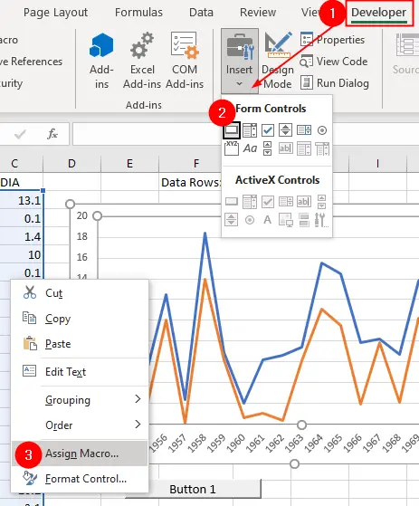
1. Go to the Developer tab. If you don’t see the Developer tab, you may need to enable Developer tab in Excel’s options.
2. Click on the Insert drop-down menu in the Controls group and select the Button (Form Control) option. Click and drag to draw the button on your worksheet.
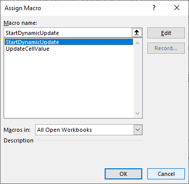
3. Right-click on the button you inserted and select Assign Macro.
4. In the Assign Macro dialog box, you should see the name of the macro you created (e.g., StartDynamicUpdate). Select the macro and click OK.
5. Close the dialog box.

Now, when you click the button, the StartDynamicUpdate macro will be executed, which will initiate the dynamic update process.

---

Charts and Graphs