You can use Excel's lookup and reference functions on a table of data to extract details corresponding to a specified value. Perhaps the most popular of these Excel functions is VLOOKUP. Although VLOOKUP is great for finding a specified value in the leftmost column of a table, you cannot use it to find the nth occurrence in the leftmost column.
You can, however, use a very simple method to find any specified occurrence you choose when using VLOOKUP, or one of the other lookup functions.
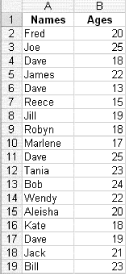
For this example, we will assume you have a two-column table of data, with column A housing first names and column B their corresponding ages, as shown in figure.
Figure. Data setup for VLOOKUP

You can use a VLOOKUP function to extract a person's age based on his name. Unfortunately, some names occur more than once. You want to be able to look up the name Dave and have the VLOOKUP function find not the first occurrence, but rather, subsequent occurrences of the name. Here is how you can do this (remember, in this example, data is in columns A and B).
First, select column A in its entirety by clicking the letter A at the column head, and then select Insert » Columns to insert a blank column (which will become column A). Click in cell A2 (skipping A1 because B1 is a heading), and enter this formula:
=B2&COUNTIF($B$2:B2,B2)
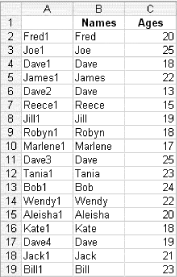
Copy this down as many rows as you have data in column B (click back in cell A2 and double-click the fill handle). You will end up with names such as Dave1, Dave2, Dave3, etc., as shown in the figure. Note the absolute reference to $B$2 in the COUNTIF function and the use of a relative reference for all references. This is vital to the function working correctly.
Figure. Data with VLOOKUP formula added to column A

If you haven't guessed already, now you can use column A as the column to find the nth occurrence of any name.
Click in cell D2 and enter in the following formula:
=VLOOKUP("Dave3",$A$1:$C$100,3,FALSE)
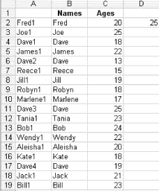
The formula will return the age for the third occurrence of the name Dave, as shown in figure.
Figure. Data with second VLOOKUP formula added to column D

You can, of course, hide column A from view, as you do not need to see it.
You also can use the names in column A as the Source range for a list in another cell by selecting Data » Validation » List. Then reference the cell housing this list in your VLOOKUP function.