ShowDetail to Filter a Recordset

The equivalent VBA property is ShowDetail. By setting this property to true for any cell in the pivot table, you will generate a new worksheet with all the records that make up that cell:

PT.TableRange2.Offset(2, 1).Resize(1, 1).ShowDetail = True

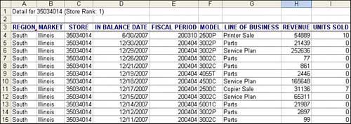
Listing 7 produces a pivot table with the total revenue for the top three stores and ShowDetail for each of those stores. This is an alternative method to using the Advanced Filter report. The results of this macro are three new sheets. Figure 19 shows the first sheet created.

Listing 7. Code That Uses the ShowDetail Method to Provide Detail for the Top Three Customers

Sub RetrieveTop3StoreDetail()
    ' Retrieve Details from Top 3 Stores
    Dim WSD As Worksheet
    Dim WSR As Worksheet
    Dim WBN As Workbook
    Dim PTCache As PivotCache
    Dim PT As PivotTable
    Dim PRange As Range
    Dim FinalRow As Long
    Set WSD = Worksheets("PivotTable")

    ' Delete any prior pivot tables
    For Each PT In WSD.PivotTables
        PT.TableRange2.Clear
    Next PT

    ' Define input area and set up a Pivot Cache
    FinalRow = WSD.Cells(Application.Rows.Count, 1).End(xlUp).Row
    FinalCol = WSD.Cells(1, Application.Columns.Count). _
        End(xlToLeft).Column
    Set PRange = WSD.Cells(1, 1).Resize(FinalRow, FinalCol)
    Set PTCache = ActiveWorkbook.PivotCaches.Add(SourceType:= _
        xlDatabase, SourceData:=PRange.Address)

    ' Create the Pivot Table from the Pivot Cache
    Set PT = PTCache.CreatePivotTable(TableDestination:=WSD. _
        Cells(2, FinalCol + 2), TableName:="PivotTable1")

    ' Turn off updating while building the table
    PT.ManualUpdate = True

    ' Set up the row fields
    PT.AddFields RowFields:="Store", ColumnFields:="Data"

    ' Set up the data fields
    With PT.PivotFields("Revenue")
        .Orientation = xlDataField
        .Function = xlSum
        .Position = 1
        .NumberFormat = "#,##0"
        .Name = "Total Revenue"
    End With

    ' Sort Stores descending by sum of revenue
    PT.PivotFields("Store").AutoSort Order:=xlDescending, _
        Field:="Total Revenue"

    ' Show only the top 3 stores
    PT.PivotFields("Store").AutoShow Type:=xlAutomatic, Range:=xlTop, _
        Count:=3, Field:="Total Revenue"

    ' Ensure that you get zeroes instead of blanks in the data area
    PT.NullString = "0"

    ' Calc the pivot table to allow the date label to be drawn
    PT.ManualUpdate = False
    PT.ManualUpdate = True

    ' Produce summary reports for each customer
    For i = 1 To 3
        PT.TableRange2.Offset(i + 1, 1).Resize(1, 1).ShowDetail = True
        ' The active sheet has changed to the new detail report
        ' Add a title
        Range("A1:A2").EntireRow.Insert
        Range("A1").Value = "Detail for " & _
            PT.TableRange2.Offset(i + 1, 0).Resize(1, 1).Value & _
            " (Store Rank: " & i & ")"
    Next i

    MsgBox "Detail reports for top 3 stores have been created."

End Sub

19. Pivot table applications are incredibly diverse. This macro created a pivot table of the top three stores and then used the ShowDetail property to retrieve the records for each of those stores.